Transition Matrix
Properties
Transition matrices are so called stochastic matrices, which means, that all entries are real values between zero and one, meaning, that each entry is a probability and a row sum equal one, meaning that the probability to jump to an arbitrary state is one
![\[ T_{i,j}\in[0,1]\]](/wiki/pub/CompMolBio/TransitionMatrix/latexe5feb2f0aba18c0bd7764903a0b47113.png)
![\[ \sum_{j=1}^{n}T_{i,j}=1.\]](/wiki/pub/CompMolBio/TransitionMatrix/latexceb9b4620807af4d0e618df0c61baabe.png)
From the sum-statement follows easlily, that there is a right eigenvector with eigenvalue of one, which is constant
![\[ \{ r_{i}\}=\{ c,c,\ldots,c\}\]](/wiki/pub/CompMolBio/TransitionMatrix/latexe2745f3af2b62b34029bcce84e658a72.png)
![\[ T_{i,j}r_{j}=r_{i}\]](/wiki/pub/CompMolBio/TransitionMatrix/latex498d2e9288424138880d25d76f3bd7fc.png)
- there exists a positive eigenvalue of one, which is called Perron Eigenvalue
- All other eigenvalues lie within the spectral radius defined by the Perron Eigenvalue
![\[|\lambda_{i}|\le1=|\lambda_{Perron}|\]](/wiki/pub/CompMolBio/TransitionMatrix/latex76078ab5c002a6ca8f5b5a1bb4cf644e.png)
- the associated left and right eigenvector are also non-negative, so also the left eigenvalue is non negativ.
- if all entries
 are strictly positive, then, the dimension of the eigenspace associated with the Perron-Eigenvalue is one.
 and sum one. That means that the probability over all states
is one. The probability in each state is then moved to other states,
when we apply this vector to the left-hand side of the transition
matrix.
For the left Perron-Eigenvalue
and sum one. That means that the probability over all states
is one. The probability in each state is then moved to other states,
when we apply this vector to the left-hand side of the transition
matrix.
For the left Perron-Eigenvalue  can be shown, that it resembles
the stationary distribution. That means, that this distribution applied
to the transition matrix does not change, i.e. it is an eigenvector
to an eigenvalue of one.
can be shown, that it resembles
the stationary distribution. That means, that this distribution applied
to the transition matrix does not change, i.e. it is an eigenvector
to an eigenvalue of one.
![\[ \pi_{i}T_{ij}=\pi_{j}\]](/wiki/pub/CompMolBio/TransitionMatrix/latex11263b6bbd2e4aefe2533ddcc00c8b83.png)
Important to know is, that the existance of the stationary distribution is not connected to the detailed balance property
Detailed balance is defined as
![\[ \pi_{i}T_{ij}=\pi_{j}T_{ji},\]](/wiki/pub/CompMolBio/TransitionMatrix/latex88c901bfcc8fc178f746364c4302cb3c.png)
which is equivalent to a symmetry over the stationary distribution.
In some cases it is possible to postulate a generator, which taken to the exponent can construct the transition matrix for arbitrary timesteps.
This is only possibile (in a unique and intuitive way), if the transition matrix is positive definite
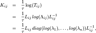
which is due to the logarithm of the eigenvalues, which are only uniquely defined, if the matrix is positive definite.
From the rate matrix we get back using
![\[ T_{ij}(\tau)=\exp(\tau\cdot K_{ij})\]](/wiki/pub/CompMolBio/TransitionMatrix/latex884fdc9a34997d3753738308e92130a9.png)